Singularity Systems: Zero to Hero

Dragon Book 2.0: The Hacker's Guide to Tensor Programs and Compilers

Singularity Systems: Zero to Hero is a SystemsML course designed for the age of heterogenous compute that powers software 2.0. This textbook spans the entire semantic chasm from the transistor to the tensor by building 4 compilers (yes four) from scratch starting from the bottom up and ending with a stack of programming languages capable of compiling the llama family of models.

Roadmap

v1.0: pretraining llama
v1.5: distributed pretraining llama
v2.0: post-training (r1) and inference systems (vllm/sglang)

Contributing

The textbook and its 4 compilers are all open source. For discussion come join us at the #singularity-systems work group in the GPU Mode Discord.

Citation

@article{j4orz2025singsys,
  author  = "j4orz",
  title   = "Singularity Systems: Zero to Hero",
  year    = "2025",
  url     = "https://j4orz.ai/zero-to-hero/"
}

Dedication

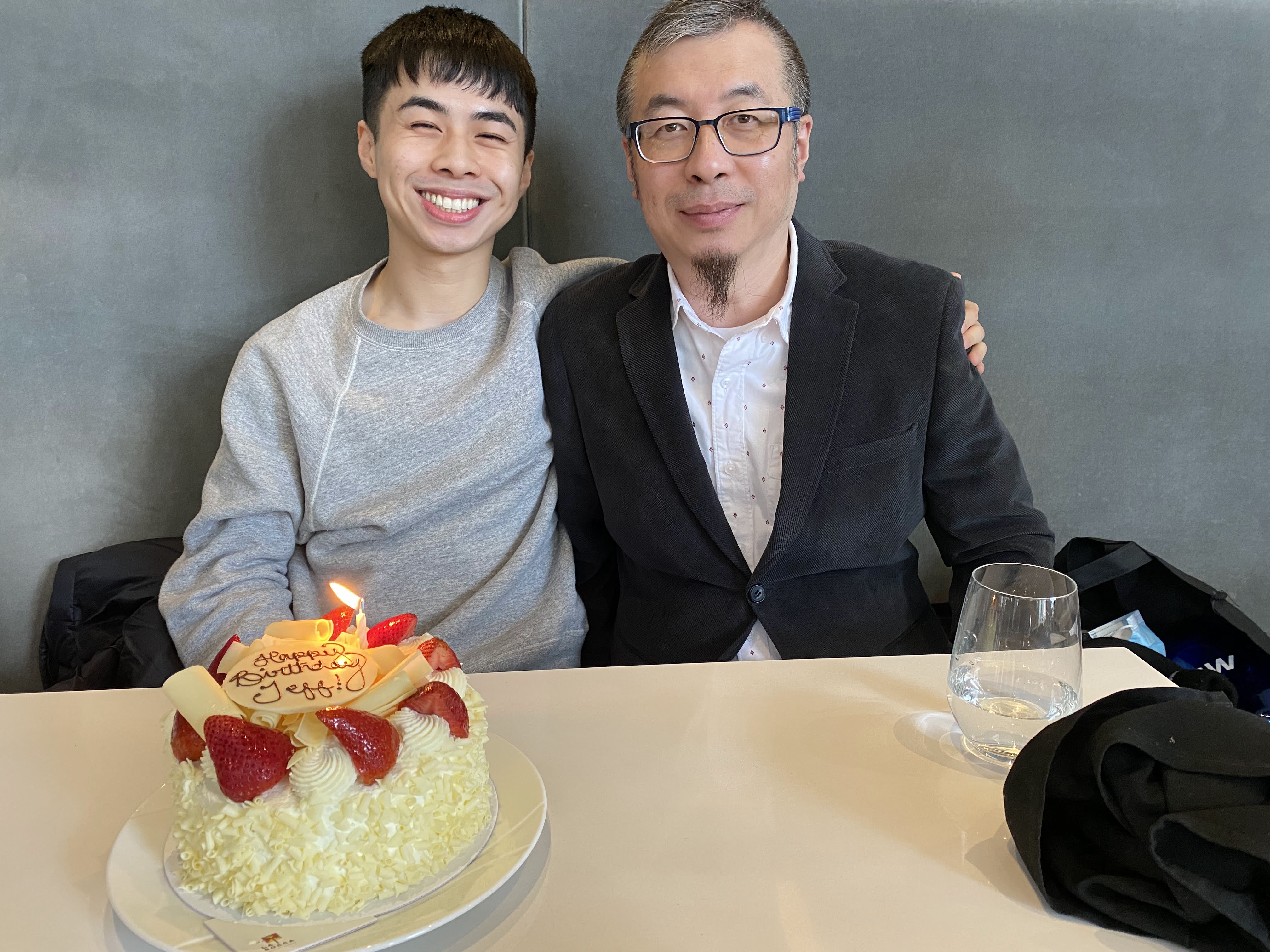
I dedicate this textbook to my father, Thomas Zhang.

In 2023, his wisdom guided me as my plans to pursue a PhD were changed to leading my sister's recovery program with her schizophrenia diagonosis. Not long after, he showed an even deeper courage of his own, meeting a severe stroke with strength, courage, and honor.

Singularity Systems Overview

Contents

• Singularity Overview
• Systems Overview

Singularity Overview — Software 2.0

Systems Overview — "Golden Age" Infrastructure Buildout

implementing 4 compilers might be intimidating. In the same way artists paint over and over, and mathematicians rederive over and over, language implementors should represent over and over.

                  ,--.    ,--.
                 ((O ))--((O ))
               ,'_`--'____`--'_`.
      _|---------------------------------|_             to the tensor
     | |Tensor Compiler: Torch  -> Triton| |                  ^
     | |Tiling Compiler: Triton -> PTX   | |                  ^
     | |Vector Compiler: CUDA   -> PTX   | |                  ^
     | |Scalar Compiler: C      -> RISC-V| |                  ^
     | |---------------------------------| |           passing assembly
     | |:::::::::::::::::::::::::::::::::| |                  ^
     | |::::::::::::::µarch::::::::::::::| |                  ^
     |_|:::::::::::::::::::::::::::::::::|_|                  ^
       |---------------------------------|           from the transistor
            __..-'            `-..__
         .-| : .----------------. : |-.
       ,\ || | |\______________/| | || /.
      /`.\:| | ||  __  __  __  || | |;/,'\
     :`-._\;.| || '--''--''--' || |,:/_.-':
     |    :  | || .----------. || |  :    |
     |    |  | || '----SSt---' || |  |    |
     |    |  | ||   _   _   _  || |  |    |
     :,--.;  | ||  (_) (_) (_) || |  :,--.;
     (`-'|)  | ||______________|| |  (|`-')
      `--'   | |/______________\| |   `--'
             |____________________|
              `.________________,'
               (_______)(_______)
               (_______)(_______)
               (_______)(_______)
               (_______)(_______)
              |        ||        |
              '--------''--------'

Course Information Singularity Systems: Zero to Hero follows up from Neural Networks: Zero to Hero. We convert

• micrograd: toy backpropagation engine into...
• picograd: modern deep learning framework

While micrograd helps research scientists to understand the leaky abstraction of backpropagation, picograd is intended for systems programmers and performance engineers looking to further understand the compilers and chips of deep learning.

Try it out with:

pip install picograd

Prerequisites

• solid deep learning (llama)
• solid systems programming (C || C++ || Rust)

Syllabus Core: Deep Learning Compilers

1. dfdx(nd): implements an interpreter for neural networks (HIPS/autograd)
2. brrr: accelerates the interpreter with vector processing (pytorch1)
3. pt2: constructs a compiler for neural networks (pytorch2)
4. az1use1: 3d parallelism

Throughout the past decade, modern day AI infrastructure has rapidly evolved to meet the needs of deep neural networks — most notably with the throughput performance of GPUs moving from TFLOPS to PFLOPS. Datacenter computing now has the goal of machines with EFLOP speeds, now that that the throughput of the fastest (non-distributed) supercomputers on TOP500 LINPACK workloads are just reaching EFLOP levels.

Although the brain is an existence proof of physics powering 20PFLOP machines with 20W, the problem with the semiconductor physics of today is two-fold:

1. instruction-level parallelism from out-of-order superscalar pipelines hits diminishing returns
2. frequency scaling is hitting against Dennard scaling's power wall

and so this free-single-thread-performance-lunch aspect to Moore's law that transitioned us across computer classes from minis to micros and from micros to mobile is "over".

As a result computer architects are moving from homogenous general hardware to heterogenous specialized hardware, which means that the complexity of extracting program performance leaks upwards from the hardware — these days, to unlock the full performance of hardware, it's the programmer's responsibility to program the vector processors in multi-core/many-core machines.

The problem with the vector processing of multi-core/many-core machines is two-fold:

1. programming model: compilers were sufficiently smart with autovectorization
2. execution model: program speedups were bound by Amdahl's law

But the industry sidestepped these problems by changing the programming model to SIMT on SIMD (CUDA) and finding domains whose execution models had more parallelism (deep neural networks).

The challenge (producing a golden age) of compiler engineers and chip architects face is to find the optimal mapping from intelligence to energy. This means creating new programming languages and machiens while minimizing the accidental complexity that naturally builds up along the way:

• The Golden Age of Compiler Design (Lattner)
• A New Golden Age for Computer Architecture (Hennessy and Patterson)

Singularity Systems

The Singularity Systems: Zero to Hero course follows up from where Neural Networks: Zero to Hero left off: we will convert micrograd into picrograd, where the main difference is that:

• micrograd is a backprop engine with scalar-support helping researchers understand that backpropagation as an abstraction is in fact leaky (gradient activations, normalizations)
• picograd leans closer towards modern day deep learning frameworks with tensor-support for both pytorch1 interpretation and pytorch2 compilation.

While picograd is more oriented towards low-level system programmers and performance engineers, this framework remains pedagogical and remains a point-wise compiler. This means that we will "only" support:

• 1 model: llama
• 1 programming model: eager
• 2 execution model: eager, graph
• 2 hardware architectures: amd cpu, nvidia gpu
• 2 precisions: fp32, tf32

Welcome to the golden age of Systems ML!

8. Tensor Compilers

This chapter implements an interpreter for neural network. By the end of this chapter, you will have a working implementation of the multidimensional array abstraction pioneered by numpy, and autodifferentiation pioneered by HIPS autograd.

Contents

1. nd: forward pass with loss = model(x)
2. dfdx(nd): backward pass with loss.backward(), opt.step()
3. ffn to gpt: lstm, rnn, gpt
4. beyond nanogpt: attention variants, kv cache, speculative decoding

References

Part 1 — nd: forward pass with loss = model(x)

The following is the model definition and inference loop for a FFN language model following (Bengio et al. 2003). The API is a 1-1 match with PyTorch — take a second to convince yourself by replacing import picograd with import torch and sampling from the inference loop.

"""
Dimension key:
B: batch size
T: sequence length
V: vocabulary size
E: embedding dimension (E != D)
D: model dimension
"""

import picograd
# from jaxtyping import

# *********************MODEL*********************
B, T = 32, 3
V, E, D = 27, 10, 200

class Linear:
  def __init__(self, D_in, D_out, bias=True):
    self.W_DiDo = picograd.randn((D_in, D_out)) * 0.01
    self.b_Do = picograd.zeros(D_out) if bias else None

  def __call__(self, X_Di):
    self.X_Do = X_Di @ self.W_DiDo
    if self.b_Do is not None: self.X_Do += self.b_Do
    self.out = self.X_Do
    return self.X_Do

  def parameters(self):
    return [self.W_DiDo] + ([] if self.b_Do is None else [self.b_Do])

class Tanh:
  def __call__(self, X_BD):
    self.X_BD = picograd.tanh(X_BD)
    self.out = self.X_BD
    return self.X_BD
  
  def parameters(self):
    return []

model = [
  Linear(T * E, D, bias=False), Tanh(),
  Linear(D, D, bias=False), Tanh(),
  Linear(D, V, bias=False)
]

C_VE = picograd.randn((V,E)) #, generator=g)
params = [C_VE] + [p for l in model for p in l.parameters()]
for p in params:
    p.requires_grad = True

print("model loaded to cpu")


# *********************INFERENCE LOOP*********************
for _ in range(20): # 20 samples
  output, context = [], [0] * T
  while True:
    X_1T = picograd.tensor([context]) # B=1 for inference, T=3, in [0..27] (set to 0 for init)
    X_1TE = C_VE[X_1T] # using 0..27 as indices into C_VE for each B=1 example of context length T
    X_1cTE = X_1TE.view(-1, T*E) # B=1, TE
    X = X_1cTE

    for h in model:
      X = h(X)

    y_hat = F.softmax(X, dim=1)

    # sample and autoregressively update context
    token = picograd.multinomial(y_hat, num_samples=1, replacement=True).item()#, generator=g).item()
    context = context[1:] + [token]
    output.append(decode[token])
    if token == 0:
        break
  print(''.join(output))

At the end of part 1 we will be able to autoregressively sample from the untrained model with the inference loop.

Contents

• Prediction, Posteriors, Parameters
  • Prediction
    • Non-parametric Inference with Posterior Updates
      • Support Vector Machines (SVMs)
      • Gaussian Processes (GPs)
      • Bayesian Linear Models
      • Bayesian Neural Networks (BNNs)
    • Parametric Inference with Parameter Estimation
      • Generalized Linear Models (GLMs): Linear and Logistic Regression
      • Deep Neural Networks (DNNs)
  • Posterior Updates
    • Probability Theory
      • Probability Space: Measurable Space + Measure
      • Discrete Random Variables: $Bin(n,p)$, $Poi(\lambda )$, $Geo(p)$
      • Continuous Random Variables: $Uni(\alpha ,\beta )$, $Exp(\lambda )$, $Nor(\mu ,{\sigma }^2)$
      • Joint Random Variables: Product Rule, Sum Rule, Bayes' Rule
    • Information Theory
      • Kullback–Leibler Divergence
      • Entropy
      • Compression
      • Algorithmic Information Theory
    • Linear Algebra
  • Parameter Estimation
    • Statistics
      • Maximum Likelihood Estimation (MLE)
      • Maximum a Posterior Estimation (MAP)
      • Empirical Risk Minimization (ERM)
    • Matrix Calculus
      • Derivatives, Gradients, and Jacobians
      • Automatic Diffrentiation: Sum Rule, Product Rule, Chain Rule
    • Optimization
      • First Order Methods: GD, SGD, Adam, Shampoo, Muon
      • Approximate Second Order Methods:
      • Second Order Methods: Newtons Method ...
• Pre-training: llama2, Post-training: r1

SAT.JUN.14 229 PREDICTION

• dnns
• theory
  • posteriors: information theory loss functions: (cross entropy. relative entropy. compression)
  • params: mle stats, param optimization is argmin(optimization) of gradient(matrix calculus)

A.1 Prediction

The primary goal of supervised machine learning is to leverage patterns from stochastic phenomena to predict quantities of interest without enumerating an entire population. That is, to recover the underlying distribution from a random sample. This is often the case with machine learning, where given dataset $D=\{({\mathbf{x}}^{(i)},{\mathbf{y}}^{(i)}):({\mathbf{x}}^{(i)},{\mathbf{y}}^{(i)})\stackrel{\text{iid}}{\sim }\mathcal{X}\times \mathcal{Y}{\}}_{i=0}^n$ with $\mathcal{X}={\mathbb{R}}^{d_{in}}$, $p(\mathbf{y}|\mathbf{x})$ needs to be recovered. The assumption of independence is the statistical questionably axiomatic counterpart to the probabilistic one of totality. While the assumption is philosophically and theoretically interesting to question with alternative probabilistic frameworks and statistical modeling, the iid assumption is a useful one to make progress in modeling. Returning to the problem setup, when $\mathcal{Y}\subseteq \mathbb{N}$, the task is classification, and when $\mathcal{Y}={\mathbb{R}}^{d_{out}}$, the task is regression.

There are a variety classes of functions that can be used to approximate $p(\mathbf{y}|\mathbf{x})$, but the primary distinction is between parametric and non-parametric models. The former have a fixed number of parameters with respect to the size of the dataset where differentiation is used to compute gradients in order to optimize loss functions. This stands in contrast to the latter which has variable number of parameters where integration is used to compute expectations in order to update posteriors. Before the start of the deep learning "revolution" in 2012 with the ImageNet "moment" the parametric/non-parametric distinction was more well known. There were primarily three "schools of thought":

• the "kernelists": proponents of support vector machines (SVMs)
• the "bayesians": proponents of gaussian processes (GPs)
• the "connectionists": proponents of neural networks (NNs)

where SVMs and GPs are non-parametric, and NNs are parametric. This chapter will cover all three, highlighting their differences and similarities, and — as usual in the artificial sciences — how this taxonification is in fact falsely trichotomous. That is, by the end of this chapter the reader should understand how SVMs/GPs are effectively shallow networks whereas NNs are deep networks, and how the former is much better understood theoretically while the latter is more successful experimentally.

todo: murphy's global/local latent distinction (with cho EBMs?)

1.1 Non-Parametric Inference with Posterior Updates

Gaussian Processes

Bayesian Logistic Regression

Bayesian Neural Networks

1.2 Parametric Inference with Parameter Estimation

Generalized Linear Models (GLMs): Linear and Logistic Regression

Linear Regression

Recall that the supervised learning problem is considered regression when $\mathcal{Y}=\mathbb{R}$. spotify dataset

The linear regression model recovers $p(Y=y|\mathbf{X}=\mathbf{x};\mathbf{w})\sim \mathcal{N}(\mu ,{\sigma }^2)$ that assumes $\mu$ is affine with respect to $x$. That is,

$$\begin{array}{rlrl}{y}^{(i)}:& ={\mathbf{w}}^{\mathsf{T}}\varphi (x^{(i)})+{ϵ}^{(i)}& & \text{[where ϵ(i)∼N(μ=0,σ2)]}\\ & ⟹{ϵ}^{(i)}=y^{(i)}-{\mathbf{w}}^{\mathsf{T}}\varphi (x^{(i)})\sim \mathcal{N}(\mu =0,{\sigma }^2)& & \\ & ⟹y^{(i)}\sim \mathcal{N}({\mathbf{w}}^{\mathsf{T}}\varphi (x^{(i)}),{\sigma }^2)& & \\ & ⟹p(y^{(i)}|x^{(i)};\mathbf{w})=\frac{1}{\sqrt{2\pi {\sigma }^2}}\exp (\frac{[y^{(i)}-{\mathbf{w}}^{\mathsf{T}}\varphi (x^{(i)}){]}^2}{2{\sigma }^2})& & \end{array}$$

where error is unbiased. expectation(e) is 0. error is model (unmodelled features im x)/data(measurement) uncertainty, then the loss is the likelihood.

With the model now defined, the parameter $\mathbf{w}$ needs to be estimated from the data $D=\{({\mathbf{x}}^{(i)},{\mathbf{y}}^{(i)}):({\mathbf{x}}^{(i)},{\mathbf{y}}^{(i)})\stackrel{\text{iid}}{\sim }\mathcal{X}\times \mathcal{Y}{\}}_{i=0}^n$. This is done by using the negatve log likelihood as the loss function $\mathcal{L}:{\mathbb{R}}^n\to \mathbb{R}$ to minimize so that $\mathcal{L}(\mathbf{w}):=-\log {\prod }_{i=1}^{n}p(y^{(i)}|{\mathbf{x}}^{(i)})$ is fixed with respect to the data $(x^{(i)},y^{(i)})$ and known variance ${\sigma }^2$:

$$\begin{array}{rlrl}{\hat{\mathbf{w}}}_{MLE}& \in \underset{\mathbf{w}\in \mathbf{W}}{\mathrm{argmin}}\mathcal{L}(\mathbf{w})& & \\ & =\mathrm{argmin}-\sum _{i=1}^n\log [\frac{1}{\sqrt{2\pi {\sigma }^2}}\exp (\frac{[y^{(i)}-{\mathbf{w}}^{\mathsf{T}}\varphi (x^{(i)}){]}^2}{2{\sigma }^2})]& & \\ & =\mathrm{argmin}-\sum _{i=1}^n\log \frac{1}{\sqrt{2\pi {\sigma }^2}}+\frac{[y^{(i)}-{\mathbf{w}}^{\mathsf{T}}\varphi (x^{(i)}){]}^2}{2{\sigma }^2}& & \\ & =\mathrm{argmin}-\sum _{i=1}^n\frac{1}{2}[y^{(i)}-{\mathbf{w}}^{\mathsf{T}}\varphi (x^{(i)}){]}^2& & \text{[by min wrt w]}\end{array}$$

where $\mathrm{argmin}$ is implemented by first evaluating the gradient $\nabla \mathcal{L}(\mathbf{w})$ and then iteratively applying gradient descent for each time step $t$, ${\mathbf{w}}^{(t+1)}:={\mathbf{w}}^t-\alpha \nabla \mathcal{L}(\mathbf{w})$.

First, evaluating the gradient $\nabla \mathcal{L}(\mathbf{w})$ looks like:

$$\begin{array}{rl}\frac{\partial \mathcal{L}(\mathbf{w})}{\partial {\mathbf{w}}_j}& =-\frac{\partial }{\partial {\mathbf{w}}_j}\sum _{i=1}^n\frac{1}{2}[y^{(i)}-{\mathbf{w}}^{\mathsf{T}}\varphi (x^{(i)}){]}^2\\ & =-\sum _{i=1}^n\frac{\partial }{\partial {\mathbf{w}}_j}\frac{1}{2}[y^{(i)}-{\mathbf{w}}^{\mathsf{T}}\varphi (x^{(i)}){]}^2\\ & =-\sum _{i=1}^n[y^{(i)}-{\mathbf{w}}^{\mathsf{T}}\varphi (x^{(i)})][-\varphi (x^{(i)}{)}_j]\end{array}$$

And so the swapping indices $j$ for the entire gradient gives $\nabla \mathcal{L}(\mathbf{w})=-{\sum }_{i=1}^n[y^{(i)}-{\mathbf{w}}^{\mathsf{T}}\varphi (x^{(i)})][-\varphi (x^{(i)})]$. Recall now that the second step in implementing $\mathrm{argmin}$ after taking $\nabla \mathcal{L}(\mathbf{w})$ is to then iteratively apply gradient descent for each time step $t$, ${\mathbf{w}}^{(t+1)}:={\mathbf{w}}^t-\alpha \nabla \mathcal{L}(\mathbf{w})$.

Logistic Regression

Recall that the supervised learning problem is considered classification when $\mathcal{Y}\subseteq \mathbb{N}$. The simple case when the output space is $\mathcal{Y}=\{-1,1\}$ is referred to as binary classification, and in the case when the output space is $\mathcal{Y}=\{0,1,\dots ,k\}$ is referred to as multi-class classification.

Many predictive values of interest that can be posed as answers to yes/no questions are suitable to be modeled as binary classifiers. For instance, benign or malignant in health care, innocent or guilty in law, real or spam in engineering. The running example used for the next two models will be the domain of music — to classifying a set of rap lyrics as a praise or diss. The set of lyrics $x^{(i)}$ that is of particular interest is Kendrick's featured verse in Kanye's "No More Parties in LA":

Hey baby you forgot your Ray Bans
And my sheets still orange from your spray tan
It was more than soft porn for the K-man
She remember my Sprinter, said "I was in the grape van"
Uhm, well cutie, I like your bougie booty
Come Erykah Badu me, well, let's make a movie
Hell, you know my repertoire is like a wrestler
I show you the ropes, connect the dots
A country girl that love Hollywood
Mama used to cook red beans and rice
Now it's Denny's, 4 in the morning, spoil your appetite
Liquor pouring and niggas swarming your section with erection
Smoke in every direction, middle finger pedestrians
R&B singers and lesbians, rappers and managers
Music and iPhone cameras
This shit unanimous for you, it's damaging for you, I think
That pussy should only be holding exclusive rights to me, I mean
He flew you in this motherfucker on first class
Even went out his way so you could check in an extra bag
Now you wanna divide the yam like it equate the math?
That shit don't add up, you're making him mad as fuck
She said she came out here to find an A-list rapper
I said baby, spin that round and say the alphabet backwards
You're dealing with malpractice, don't kill a good nigga's confidence
Just cause he a nerd and you don't know what a condom is
The head still good though, the head still good though
Make me say "Nam Myoho Renge Kyo"
Make a nigga say big words and act lyrical
Make me get spiritual
Make me believe in miracles, Buddhist monks and Cap'n Crunch cereal
Lord have mercy, thou will not hurt me
Five buddies all herded up on a Thursday
Bottle service, head service, I came in first place
The opportunity, the proper top of breast and booty cheek
The pop community, I mean these bitches come with union fee
And I want two of these, moving units through consumer streets
Then my shoe released, she was kicking in gratuity
And yeah G, I was all for it
She said K Lamar, you kind of dumb to be a poet
I'mma put you on game for the lames that don't know they're a rookie
Instagram is the best way to promote some pussy

The sentiment of "No More Parties in LA" is extremely difficult for a machine to classify correctly due to Kendrick's wordplay, double entendres, and insinuations. Consider the positive/negative dictionaries where positive={baby, cutie, love, good, spiritual, miracles, buddhist, buddies, opportunity, promote} and negative={shit, spoil, damaging, motherfucker, mad, fuck, malpractice, kill, mercy, hurt, fee, dumb}. Then a possible feature extractor $\varphi :\mathcal{X}\to {\mathbb{R}}^3$ which maps raw input to dimensioned feature representation is defined by:

Now that the input space $\mathcal{X}$, feature extractor $\varphi :\mathcal{X}\to {\mathbb{R}}^3$, and output space $\mathcal{Y}=\{-1,1\}$ is defined, the goal is to select some function $f:\mathcal{X}\to \mathcal{Y}$.

todo: use regression. motivate the need for the range to be a p \in [0,1]

Logistic Regression

The logistic regression model is a discriminative $p(Y=y|\mathbf{X}=\mathbf{x};\theta )\sim Ber(p)$ with a decision boundary $k\in [0,1]$ (in the case of $Ber(p)$, $k$ is usually set to $0.5$ so as to divide the mass by 2) that assumes that the parameter $p$ is affine with respect to $x$. That is, $$\begin{array}{rlrl}p(Y=1\mid \mathbf{X}=\mathbf{x})& =p:=\sigma ({\mathbf{w}}^{\mathsf{T}}\varphi (x))& & \text{[ϕ(x)0=1]}\\ ⟹p(Y=-1\mid \mathbf{X}=\mathbf{x})& =1-p=1-\sigma ({\mathbf{w}}^{\mathsf{T}}\varphi (x))& & \\ ⟹p(Y=y\mid \mathbf{X}=\mathbf{x})& =p^y(1-p{)}^{1-y}& & \\ & =\sigma ({\mathbf{w}}^{\mathsf{T}}\varphi (x){)}^y[1-\sigma ({\mathbf{w}}^{\mathsf{T}}\varphi (x)){]}^{1-y}& & \end{array}$$

where $\sigma :\mathbb{R}\to [0,1]$ is a non-linear function $\sigma :=\frac{1}{1+\exp (-z)}$, and where ${\mathbf{w}}^{\mathsf{T}}\varphi (\mathbf{x})$ is referred to as the logit since the inverse ${\sigma }^{-1}:=\log \frac{p}{1-p}$ is defined as the log odds ratio.

With the model now defined, the parameter $\mathbf{w}$ needs to be estimated from the data $D=\{({\mathbf{x}}^{(i)},{\mathbf{y}}^{(i)}):({\mathbf{x}}^{(i)},{\mathbf{y}}^{(i)})\stackrel{\text{iid}}{\sim }\mathcal{X}\times \mathcal{Y}{\}}_{i=0}^n$. This is done by using the negatve log likelihood as the loss function $\mathcal{L}:{\mathbb{R}}^n\to \mathbb{R}$ to minimize so that $\mathcal{L}(\mathbf{w}):=-\log {\prod }_{i=1}^{n}p(y^{(i)}|{\mathbf{x}}^{(i)})$ is fixed with respect to the data $(x^{(i)},y^{(i)})$

$$\begin{array}{rl}{\hat{\mathbf{w}}}_{MLE}& \in \mathrm{argmin}\mathcal{L}(\mathbf{w})\\ & =\mathrm{argmin}-\sum _{i=1}^n\log \sigma ({\mathbf{w}}^{\mathsf{T}}\varphi (x^{(i)}){)}^{y^{(i)}}[1-\sigma ({\mathbf{w}}^{\mathsf{T}}\varphi (x^{(i)})){]}^{1-y^{(i)}}\\ & =\mathrm{argmin}-\sum _{i=1}^n{y}^{(i)}\log \sigma ({\mathbf{w}}^{\mathsf{T}}\varphi (x^{(i)}))+(1-y^{(i)})\log \sigma ({\mathbf{w}}^{\mathsf{T}}\varphi (x^{(i)}))\end{array}$$

where todo kl->ce.

where $\mathrm{argmin}$ is implemented by first evaluating the gradient $\nabla \mathcal{L}(\mathbf{w})$ and then iteratively applying gradient descent for each time step $t$, ${\mathbf{w}}^{(t+1)}:={\mathbf{w}}^t-\alpha \nabla \mathcal{L}(\mathbf{w})$.

First, to evaluate the gradient, $\nabla \mathcal{L}(\mathbf{w})$, the negative log likelihood as loss function is simplified by defining ${\hat{y}}^{(i)}:=\sigma ({\mathbf{w}}^{\mathsf{T}}\varphi (x^{(i)}))$ so that $\nabla \mathcal{L}(\mathbf{w})=-{\sum }_{i=1}^n{y}^{(i)}\log {\hat{y}}^{(i)}+(1-y^{(i)})\log {\hat{y}}^{(i)}$. Note that $\hat{y}$ is not the target label but the probability of the target label. Then, since the derivative is linear with the derivative of the sum is the sum of the derivatives where $\frac{\partial }{\partial \mathbf{w}}{\sum }_{i=1}^{n}f(\mathbf{w})={\sum }_{i=1}^n\frac{\partial }{\partial \mathbf{w}}f(\mathbf{w})$, taking the derivative for a single example $i\in \{1,\dots ,n\}$ for a single parameter ${\mathbf{w}}_j$ where $\mathcal{L}(\mathbf{w})=y\log \hat{y}+(1-y)\log \hat{y}$ looks like

$$\begin{array}{rlrl}\frac{\partial \mathcal{L}(\mathbf{w})}{\partial {\mathbf{w}}_j}& =\frac{\partial \mathcal{L}(\mathbf{w})}{\partial \hat{y}}\frac{\partial \hat{y}}{\partial {\mathbf{w}}_j}& & \text{[by chain rule]}\\ & =\frac{\partial \mathcal{L}(\mathbf{w})}{\partial \hat{y}}\hat{y}(1-\hat{y})\varphi (x{)}_j& & \text{[by dzdσ=σ(1−σ)]}\\ & =[\frac{y}{\hat{y}}-\frac{1-y}{1-\hat{y}}]\hat{y}(1-\hat{y})\varphi (x{)}_j& & \text{[by dxdlog(x)=x1]}\\ & =\left[\frac{y(1-\hat{y})-\hat{y}(1-y)}{\hat{y}(1-\hat{y})}\right]\hat{y}(1-\hat{y})\varphi (x{)}_j& & \\ & =[y(1-\hat{y})-\hat{y}(1-y)]\varphi (x{)}_j& & \\ & =(y-\hat{y})\varphi (x{)}_j& & \end{array}$$

and so the evaluating the derivative of all examples $\nabla \mathcal{L}(\mathbf{w})=-{\sum }_{i=1}^n{y}^{(i)}\log {\hat{y}}^{(i)}+(1-y^{(i)})\log {\hat{y}}^{(i)}$ where ${\hat{y}}^{(i)}:=\sigma ({\mathbf{w}}^{\mathsf{T}}\varphi (x^{(i)}))$ looks like

$$\begin{array}{rl}\frac{\partial \mathcal{L}(\mathbf{w})}{\partial {\mathbf{w}}_j}& =-\sum _{i=1}^n\frac{\partial }{\partial {\mathbf{w}}_j}[y^{(i)}\log {\hat{y}}^{(i)}+(1-y^{(i)})\log {\hat{y}}^{(i)}]\\ & =-\sum _{i=1}^n(y^{(i)}-{\hat{y}}^{(i)})\varphi (x^{(i)}{)}_j\\ & =-\sum _{i=1}^n(y^{(i)}-\sigma ({\mathbf{w}}^{\mathsf{T}}\varphi (x^{(i)}))]\varphi (x^{(i)}{)}_j\end{array}$$

And so the swapping indices $j$ for the entire gradient gives $\nabla \mathcal{L}(\mathbf{w})=-{\sum }_{i=1}^n(y^{(i)}-\sigma ({\mathbf{w}}^{\mathsf{T}}\varphi (x^{(i)}))]\varphi (x^{(i)})$. Recall now that the second step in implementing $\mathrm{argmin}$ after taking $\nabla \mathcal{L}(\mathbf{w})$ is to then iteratively apply gradient descent for each time step $t$, ${\mathbf{w}}^{(t+1)}:={\mathbf{w}}^t-\alpha \nabla \mathcal{L}(\mathbf{w})$.

Multinomial Logistic Regression

GLM: $\mathcal{N}(\mu ,{\sigma }^2)$ and $Ber(p)$ is $Exp()$

sigmoid justification

• nice derivative \frac{d\sigma}{d?} = \sigma(1-\sigma) (which helps with calculus -> optimization -> parameter estimation)
• glms justify the choice of logistic/sigmoid non-linear squashing function 1/1+exp(-z).

Deep Neural Networks (DNNs)

which apriori seems difficult to learn a useful mapping for, given that the first and second dimension of the feature representation which respectively encode positive/negative sentiment are roughly tied. For instance, what is the feature extractor that maps the following set of lyrics (with subtle insinuations) into a useful feature representation for a sentiment classifier?

A country girl that love Hollywood
Mama used to cook red beans and rice
Now it's Denny's, 4 in the morning, spoil your appetite
Liquor pouring and niggas swarming your section with erection

The short answer is that it's difficult because the concept and negative sentiment becomes apparent after reading the entire paragraph rather than any specific word. This is the motivation for representation learning.

A.2 Posterior Updates

Probability Theory

By default, mathematical reasoning is understood to be deterministic where a statement $S$ is either true (holds) or false (does not hold). Any variable $x$ can only take on one specific value at a time. However there are other times where what's desirable is describing phenomena that is in fact non-deterministic (while still remaining precise). Even if base reality is fundamentally deterministic, in practice there are many scenarios where carrying out calculation is intractable. i.e, predicting tomorrow's weather with the position of every water molecule.

The most widely adopted mathematical language for formalizing our intuitions around non-deterministic stochastic phenomena is probability theory (as opposed to alternative frameworks such as probabilistic logic or uncertainty quantification). In probability theory statements $S$ are neither true nor false. Rather, truth is distributed across a weighted set of random events $E$. Similarly, random variables $X$ and their probability distributions $p$ do not take on definite values but rather sets of values. Probability theory is the generalization of aristotelian logic.

Probability Space: Measurable Space + Measure

These three concrete implementations create the toolbox which serve as workhorses for probability theory and require an abstract interface. The Kolmogorov's 1933 formulation of probability theory in Grundbegriffe der Wahrscheinlichkeitsrechnung is the universally accepted model for random events and random variables. The guiding light in the axiomaticization are the first two out of three properties that $p$ should satisfy: non-negativity and normalization, which formalize impossible (surely false) and guaranteed (surely true) statements. They ensure that probabilities are never less than 0 nor greater than 1.

The foundations start with an ambient sample space $\Omega$ which is the set of all possible outcomes $\omega$ in an experiment. It's natural to expect the probability function $p$ to be defined on $\Omega$, which is acceptable when the sample space is countable. That is, when $|\Omega |<{\aleph }_1$, the first two properties are possible to satisfy:

• non-negativity: $\forall \omega \in \Omega ,P(\omega )>0.$
• normalization: $\sum _{i=0}^{\infty }P({\omega }_i)=1.$

but when the sample space is infinitely uncountable then normalization is not possible. That is, when $|\Omega |={\aleph }_1$, TODO... The next approach then is to define probabilities for the powerset $\mathcal{F}=2^{\Omega }$ with $p:\mathcal{F}\to [0,1]$. The powerset $F$ is the set of all subsets, and is referred to as the event space. The event space must be a field. That is, it must be closed under union, intersection, and complement, satisfying:

• $\varnothing \in \mathcal{F}\wedge \Omega \in \mathcal{F}$.
• $A\in \mathcal{F}⟹\Omega \setminus A\in \mathcal{F}$.
• $A\in \mathcal{F}\wedge B\in \mathcal{F}⟹A\cup B\in \mathcal{F}\wedge A\cap B\in \mathcal{F}$.

This formulation of $p$ is now defined on $E\subset \Omega$ but still does not support sample spaces where $|\Omega |={\aleph }_1$ let alone $|\Omega |={\aleph }_0$. The property of closure of union and intersection need to be extended to support sample spaces that are countable and uncountable infinite. Starting with the former, a field $F$ that satisfies

• $E_1,E_2,\dots \in \mathcal{F}⟹\bigcup _{i=1}^{\infty }{E}_i\in \mathcal{F}\wedge \bigcup _{i=1}^{\infty }\in \mathcal{F}$.

is then a $\sigma$-field and is defined for $|\Omega |={\aleph }_0$. This $\sigma$-field with the sample space $\Omega$ form a measurable space. Finally, the original goal that motivated the need to redefine $p$'s domain from $\Omega$ to $\mathcal{F}=2^{\Omega }$ was to support uncountable infinities where $|\Omega |={\aleph }_1$. This motivates the need to add additional properties the event space must satisfy which is... this is a borel sigma field.

Returning to the probability function $p$, the original first two properties are satisified, in addition to a third and final one:

• non-negativity: $\forall \omega \in \Omega ,P(\omega )>0.$
• normalization: $\sum _{i=0}^{\infty }P({\omega }_i)=1.$
• additivity:

A measurable sapce $(\Omega ,\mathcal{F})$ with a measurable function $p:\mathcal{F}\to [0,1]$ is the abstract model for a probability space.

Example 1: finite probability space

In the notebook's running example, consider describing a rappers vocabulary as some sample space $\Omega =\{acid,balls,chop,death,grind,mind,poppin,pills,razor,shallow,tequila,zoey\}$, and the following probability assignment (take a moment to confierm that they are all non-negative and normalize to 1).

• $P(\{acid\})=0.04$
• $P(\{balls\})=0.01$
• $P(\{chop\})=0.09$
• $P(\{death\})=0.08$
• $P(\{grind\})=0.08$
• $P(\{mind\})=0.05$
• $P(\{poppin\})=0.04$
• $P(\{pills\})=0.19$
• $P(\{razor\})=0.03$
• $P(\{shallow\})=0.22$
• $P(\{tequila\})=0.15$
• $P(\{zoey\})=0.02$

Let $X:\Omega \to \mathbb{R}$ be the r.v that maps words to their lengths, and let $Y:\Omega \to \mathbb{R},$ be the r.v that maps the word $\omega$ to the ordinal-based unicode number of the first letter

• the rv taking on value $X=5$ constructs the event modeled by the subset $A=\{balls,death,grind,pills,razor\}$ and the p
• the rv taking on value $Y=112$ constructs the event modeled by the subset $B=\{poppin,pills\}$

The event where $X=5$ and $Y=112$ constructs the subset $C=A\cup B=\{pills\}$. The event where $X=5$ or $Y=112$ constructs the subset $C=A\cap B=\{balls,death,grind,poppin,pills,razor\}$

Example 2: continuous probability space

Discrete Random Variables

Continuous Random Variables

Rulez Rule: Product Rule, Sum Rule, Bayes' Rule

With an axiomaticization in place where random events $E$ and random variables $X$ are modeled as measurable subsets and measurable functions of a measurable space $\Omega$, the focus is now on the core — invariant to sample space modifications — probabilistic concepts that comprise the notion of updating beliefs.

It all starts with of conditional probability, which is the probability of some event $A$ given that event $B$ was observed. If the Kolmogorov axiomaticization admits modeling stochastic events $A$ and $B$ as a venn diagram within an ambient sample space, then conditional probability changes the fidelity of description so that $B$ is the new (and narrowed) "sample space" being considered. That is, probability of $A$ given $B$ is denoted with $P(A\mid B)$ and is defined as

$$P(A\mid B)\stackrel{△}{=}\frac{P(A\cap B)}{P(B)}$$

and can itself be proved a valid probability space. In other scenarios $P(A\mid B)$ is given, but $P(A\cap B)$ is not. This is amenable by rearranging the definition and solving for the latter with $P(A\cap B)=P(B)P(A\mid B)$. and is referred to as the product rule (emphasis on the product) or chain rule (emphasis on the factors).

In other scenarios $P(A\mid B)$ is given (and now $P(A\cap B)$ by the product rule), but $P(A)$ is not. This too is amenable by using event $B$ as a "background event", where assuming events $B_1,B_2,\dots B_n$ are mutually exclusive, then $P(A)=P(A\cap B_1)+P(A\cap B_2)+\dots +P(A\cap B_N)$. This is referred to as the sum rule, and can be composed with the product rule to further decompose the terms of products into terms of conditionals.

Finally, in other scenarios where $P(A\mid B)$ is given but $P(B\mid A)$ is not, this is amenable by rewriting the numerator and denominator of conditional probability using the product rule and sum rule:

$$\begin{array}{rlrl}P(A\mid B)& =\frac{P(A\cap B)}{P(B)}& & \text{[by definition of conditional]}\\ & =\frac{P(A)P(B\mid A)}{P(B)}& & \text{[by product rule on joint]}\end{array}$$

$$\underset{\text{posterior}}{\underbrace{p(x\mid y)}}=\frac{\stackrel{\text{likelihood}}{\overbrace{p(y\mid x)}}\stackrel{\text{prior}}{\overbrace{p(x)}}}{\underset{\text{evidence}}{\underbrace{\int p(y\mid x)p(x)dx}}}.$$

and is referred to as bayes' rule. The scenario where $P(A\mid B)$ is accessible but $P(B\mid A)$ is not comes up many times practice, where $A$ is some latent event and $B$ is an observable event. This happens in science (why bayes rule is also referred to as the logic of science) where $P(A\mid B)$ is used to model hypothesis and evidence where the posterior $P(H\mid E)$ (latent given observed) is updated by evaluating the product of the prior $P(H)$ and the likelihood (observed given latent) $P(E\mid H)$ normalized by the evidence $P(E)$.

Example 3: conditional probability

Let $\Omega$ be the sample space used from the previous examples, $Y:\Omega \to \mathbb{R}$ once again be the r.v that maps the word $\omega$ to the ordinal-based unicode number of the first letter, and let $Z:\Omega \to \mathbb{R}$ be a new identity r.v $Z$ that maps the word to it's hash. What's $P(Z=hash("pills")|Y=112)$? The answer by definition of conditional probability is $\frac{0.19}{0.04+0.19}=0.83$, where $P(Y=112)=0.04+0.19$ because of additivity.

todo: examples 4/5/6: product rule/sum rule/bayes rule

Inference: Joint Random Variables

from jax import numpy as jnp
from jaxtyping import Array, Float

def bayes(joint: Float[Array, "dx dy"]) -> Float[Array, "dx dy"]:
    prior = 0
    likelihood = 0
    evidence = 0

    posterior = 0
    return prior, likelihood, evidence, posterior

Information Theory

Kullback-Leibler Divergence

Entropy

Compression

Algorithmic Information Theory

A.3 Parameter Estimation

Statistics

In probabilistic models distributions of latent hypotheses are usually unknown and their posteriors are inferred with bayes rule by taking the product of the prior $p(h)$, likelihood $p(e,h)$, and normalizing by the evidence $p(e)$. When these latter distributions (more specifically, the parameters $\theta$ that characterize them), the parameters need to be recovered from data via parameter estimation.

Empirical Risk Minimization (ERM)

Risk is a quantity where the objective is to minimize. Reward is a quantity where the objective is to maximize.

loss functions and risk.

• theta_likelihood from L_likelihood (likelihood from the probabilistic perspective)
• theta_0-1 from L_01
• theta_absolute from L_abs

Unbiased Estimators

Maximum Likelihood Estimation (MLE)

Maximizing the likelihood uses the probability model itself as the loss function. Following the notion of minimizing risk, the maximization corresponds to minimizing the negative likelihood $-p(x;\theta )$. One more transformation is applied by mapping the likelihood to log space which simplifies the $\mathrm{argmin}$ routine by decomposing the joint probability of the data $p(x_1,x_2,\dots ,x_n;\theta )$ into a product of likelihoods with the chain rule (assuming $X_1,X_2,\dots ,X_N\stackrel{\text{iid}}{\sim }p$). The parameters which minimize negative log likelihood are the same that minimize negative likelihood since logarithms perserve monotonicity. All together, the optimization problem is:

$$\begin{array}{rlrl}\hat{\mathbf{\theta }}& \in \underset{\mathbf{\theta }\in \Theta }{\mathrm{argmax}}p(x;\theta )& & \\ & =\mathrm{argmax}\log p(x_1,x_2,\dots ,x_n;\theta )& & \text{[by monotonicity of log]}\\ & =\mathrm{argmin}-\log p(x_1,x_2,\dots ,x_n;\theta )& & \\ & =\mathrm{argmin}-\log \prod _{i=1}^{n}p(x_i;\theta )& & \text{[by Xi∼iidp]}\\ & =\mathrm{argmin}-\sum _{i=1}^n\log p(x_i;\theta )& & \text{[by log laws]}\end{array}$$

In the following examples $\mathrm{argmin}$ is implemented symbolically by solving for $\frac{d}{d\theta }=0$.

Example 1: maximizing likelihood with $Poi(\lambda )$

Assume $X_1,X_2,\dots ,X_n\stackrel{\text{iid}}{\sim }Poi(\lambda ).$ Then using negative log likelihood as the loss function corresponds to the following optimization:

$$\begin{array}{rl}{\hat{\lambda }}_{MLE}& \in \mathrm{argmin}\mathcal{L}(\lambda )\\ & =\mathrm{argmin}-\sum _{i=1}^n\log \frac{e^{-\lambda }{\lambda }^{x_i}}{x_i!}\\ & =\mathrm{argmin}-\sum _{i=1}^n-\lambda +x_i\log \lambda -\log x_i!\end{array}$$

and solving for the arguments $\lambda$ which minimize the expression corresponds to taking the derivative with respect to $\lambda$ and solve for those that equal 0:

$$\begin{array}{rl}\frac{\partial \mathcal{L}}{\partial \lambda }& =0\\ -\sum _{i=1}^n-1+\frac{x_i}{\lambda }& =0\\ n-\frac{1}{\lambda }\sum _{i=1}^n{x}_i& =0\\ \frac{1}{n}\sum _{i=1}^n{x}_i& ={\lambda }_{MLE}\end{array}$$

Example 2: maximizing likelihood with $Ber(p)$

Assume $X_1,X_2,\dots ,X_n\stackrel{\text{iid}}{\sim }Ber(p).$ Then using negative log likelihood as the loss function corresponds to the following optimization:

$$\begin{array}{rl}{\hat{p}}_{MLE}& \in \mathrm{argmin}\mathcal{L}(p)\\ & =\mathrm{argmin}-\sum _{i=1}^n\log [p^{x_i}(1-p{)}^{1-x_i}]\\ & =\mathrm{argmin}-\sum _{i=1}^n{x}_i\log p+(1-x_i)\log (1-p)\end{array}$$

and solving for the arguments $p$ which minimize the expression corresponds to taking the derivative with respect to $p$ and solve for those that equal 0:

$$\begin{array}{rlrl}\frac{\partial \mathcal{L}}{\partial p}& =0& & \\ \frac{\partial \mathcal{L}}{\partial p}-\sum _{i=1}^n{x}_i\log p+(1-x_i)\log (1-p)& =0& & \\ \frac{\partial \mathcal{L}}{\partial p}-[X\log p+(n-X)\log (1-p)]& =0& & \text{[where X=∑i=1nxi]}\\ \frac{-X}{p}+\frac{n-X}{1-p}& =0& & \\ -X+Xp+np-Xp& =0& & \\ np& =X& & \\ p_{MLE}& =\frac{1}{n}\sum _{i=1}^n{x}_i& & \end{array}$$

Example 3: maximizing likelihood with $Nor(n,{\sigma }^2)$

Assume $X_1,X_2,\dots ,X_n\stackrel{\text{iid}}{\sim }Nor(\mu ,{\sigma }^2).$ Then using negative log likelihood as the loss function corresponds to the following optimization:

$$\begin{array}{rlrl}{\hat{\theta }}_{MLE}& \in \mathrm{argmin}\mathcal{L}(\theta )& & \text{[where θ=(μ,σ2)]}\\ & =\mathrm{argmin}-\sum _{i=1}^n\log [p^{x_i}(1-p{)}^{1-x_i}]& & \end{array}$$

and solving for the arguments $p$ which minimize the expression corresponds to taking the derivative with respect to $p$ and solve for those that equal 0:

$$\begin{array}{rlrl}\frac{\partial \mathcal{L}}{\partial p}& =0& & \\ \frac{\partial \mathcal{L}}{\partial p}-\sum _{i=1}^n{x}_i\log p+(1-x_i)\log (1-p)& =0& & \\ \frac{\partial \mathcal{L}}{\partial p}-[X\log p+(n-X)\log (1-p)]& =0& & \text{[where X=∑i=1nxi]}\\ \frac{-X}{p}+\frac{n-X}{1-p}& =0& & \\ -X+Xp+np-Xp& =0& & \\ np& =X& & \\ p_{MLE}& =\frac{1}{n}\sum _{i=1}^n{x}_i& & \end{array}$$

Maximum a Posterior Estimation (MAP)

Matrix Calculus

Recall that for some scalar function $f:\mathbb{R}\to \mathbb{R}$ that the derivative is usually defined as $\frac{df}{dx}=f^{\prime }(x)$ where the derivative $f^{\prime }(x)$ is the ratio between the differentials (inifinitesmal differences) of input $dx$ and output $df$. While $/:\mathbb{R}\to \mathbb{R}$ is defined on $\mathbb{R}$, this is not always the case for higher dimensional euclidean spaces.

Moreover, the problem with the formulation of derivatives as $\frac{df}{dx}$ is not limited to denotational semantic lawyering — there's also a problem with the derivative rules themselves. Consider the function $f:{\mathbb{R}}^{n\times n}\to {\mathbb{R}}^{n\times n}$, $f(\mathbf{X}):={\mathbf{X}}^2$ which squares a matrix. The power rule of scalar functions does not generalize here, because $f^{\prime }(x)\ne 2\mathbf{X}$.

Defining $f^{\prime }(x)$ as a ratio $f^{\prime }(x)=\frac{df}{dx}$ does not generalize. Instead, the correct approach is to define the derivative as linearization which defines the derivative as the linear operator you apply to a change in output to receive a change in output. That is, $df=f^{\prime }(x)dx$. This formulation of the derivative generalizes scalar and vector differential calculus over $\mathbb{R}$ and ${\mathbb{R}}^n$ into higher dimensional vector spaces for matrix and tensor calculus over ${\mathbb{R}}^{n\times m}$ and ${\mathbb{R}}^{d_0\times d_1\cdots \times d_n}$. In essence, linearization is locally approximating complex surfaces in vector spaces $\mathcal{V}$ (more specifically, Banach spaces equipped with norm $||x||$) with linear operators $L:\mathcal{V}\to \mathcal{V}$ ($L[v_1+v_2]=L[v_1]+L[v_2]$) so that $\Delta \text{out}=L[\Delta \text{in}]$.

Derivatives, Gradients, and Jacobians

• for some function $f:\mathbb{R}\to \mathbb{R}$, $f^{\prime }(x)$ is the term such that $df=f^{\prime }(x)[dx]$. For this expression to be defined, $dx\in \mathbb{R}\wedge df\in \mathbb{R}⟹f^{\prime }(x)\in \mathbb{R}\wedge [\bullet ]:=\ast$ where $\ast :\mathbb{R}\to \mathbb{R}$.
• for some function $f:{\mathbb{R}}^n\to \mathbb{R}$, $f^{\prime }(\mathbf{x})$ is the term such that $df=f^{\prime }(\mathbf{x})[d\mathbf{x}]$. For this expression to be defined, $d\mathbf{x}\in {\mathbb{R}}^n\wedge df\in \mathbb{R}⟹f^{\prime }(\mathbf{x})\in {\mathbb{R}}^n\wedge [\bullet ]:=\cdot$ where $\cdot :{\mathbb{R}}^n,{\mathbb{R}}^n\to \mathbb{R}$. In this case, $f^{\prime }(\mathbf{x})$ is often referred to as the gradient of $f$ and denoted by $\nabla f$
• for some function $f:{\mathbb{R}}^n\to {\mathbb{R}}^m$, $f^{\prime }(\mathbf{x})$ is the term such that $d\mathbf{f}=f^{\prime }(\mathbf{x})[d\mathbf{x}]$. For this expression to be defined, $d\mathbf{x}\in {\mathbb{R}}^n\wedge d\mathbf{f}\in {\mathbb{R}}^m⟹f^{\prime }(\mathbf{x})\in {\mathbb{R}}^{m\times n}\wedge [\bullet ]:=@$ where $@:{\mathbb{R}}^n\to {\mathbb{R}}^m$. In this case, $f^{\prime }(\mathbf{x})$ is often referred to as the jacobian of $f$ and denoted by $Jf$

numerical example.

Automatic Differentiation

as opposed to symbolic or numerical.

Optimization

Gradient Descent

Stochastic Gradient Descent

Adam

Shampoo

Muon

and more generally we define the derivative as the linear operator L on vector space V which you apply to a change in input in order to obtain the change in output. That is, Δout = (lin.op)[Δin]. which generalizes to higher dimensions. While defining f'x ≜ df/dx is legal when f: ℝ -> ℝ, it's usually not clear what df/dx means in higher dimensions, since /: ℝ^n, R^m -> ? is not defined.

f: ℝ^d -> ℝ

Consider f'(x) when f: ℝ^d -> ℝ. Then, given that dx ∈ ℝ and df ∈ ℝ^d, the linear operator f'(x) must (formalized by the Riecz-Frchét Representation Theorem) be the dot product with some column vector, (multiplication with the column vector transposed). Let's call this column vector the "gradient" of f, where the component-wise definition with indices is:

    ∇f ∈ ℝ^d, f'(x) = ∇fᵀx
    ∇f_i ≜ ∂f/∂x_i ∀ i ∈ [0..d]
and all together, we use f'(x) to linearize df:
    f(x+dx)-f(x) = df
                 = f'(x)dx
                 = ∇fᵀdx

f: ℝ^m -> ℝ^n

Moving on, consider f'(x) where f: ℝ^m -> ℝ^n. Then given that dx ∈ ℝ^m and df ∈ ℝ^n, the linear operator f'(x) must (formalized by the Riecz-Frchét Representation Theorem once again) expressable as a matrix multiplication with some matrix A ∈ ℝ^(mxn). Let's call this matrix the "jacobian", where the component-wise definition with indices is the following:

    Jf ∈ ℝ^(nxm), f'(x) = Jdx
    Jf_ij ≜ ∂fi/∂xj ∀ i ∈ [0..n], j ∈ [0..m]
and all together, we use f'(x) to linearize df:
    f(x+dx)-f(x) = df
                 = f'(x)dx
                 = Jdx

f: ℝ^m, ℝ^n -> ℝ^p [f: ℝ^(nxm), ℝ^(mxp) -> ℝ^(nxp)]

For example, given f: ℝ^m -> ℝ^n, f(x) := Ax

==> df = f(x+dx)-f(x)
       = (Ax+dx)-Ax
       = Adx
==> f'(x) = A = J

While it's very elegant that the derivative of Ax turns out to be A, training neural networks requires that is A is not just constant, but variable with respect to f. To make the deep learning context clearer, we will use W instead of A:

  fi(W,x) ≜ ΣWij*xj
    f(x) := [f1(x), f2(x), ..., fn(x)]
but we can just promote x to be a matrix too. Finally, consider f'(x) when
f: ℝ^(nxm), ℝ^(mxp) -> ℝ^(nxp)

ℒ: ℝ^d0 -> ℝ ∋ ℒ(Z) where Z := X @ Y
==> dℒ = dℒ/dZ : dZ                             [by Riecz. Representation Theorem]
       = dℒ/dZ : (dX@Y + X@dY)                  [by product rule on dZ]
       = dℒ/dZ : (dX@Y) + dℒ/dZ : (X@dY)        [: linear]
       = (dℒ/dZ@Yᵀ) : dX + (Xᵀ@dℒ/dZ) : dY      [by TODO...circularity of trace]                              
==> dℒ/dX = dℒ/dZ@Yᵀ ∧ dℒ/dY = Xᵀ@dℒ/dZ

Stepping back, defining the derivative this way generalizes the rise over run with scalars, the gradient with vectors, and the jacobian with matrices into the same notion: they are the linear operators defined on vector spaces that you apply to a change in input in order to obtain the change in output, and the types/shapes are defined the way they are out of necessity, rather than by fiat. Moreover, this also sharpens the semantics of the denotation in higher dimensions given that df/dx is often ill-defined. i.e. while df/dx makes sense when df, dx ∈ ℝ^n, dividing tensors with mismatched shapes becomes nonsensical.

This also means that this definition extends to any vector space where a linear operator is defined, for instance, the space of matrices (vectorization of matrices), and the space of functions (calculus of variations).

While training deep neural networks do not involve functions that map matrices to matrices or functions to functions, defined this way it's clear that many of the "grads" we take in pytorch are actually jacobians that all compose into one single gradient for the entire expression graph which represents some function f: ℝ^n -> ℝ.

2b — Derivative rules: backward methods

defining rules for any f: V->V

Sum rule
--------
f: V -> V
f(x) := g(x) + h(x)
==>      df = dg + dh
    f'(x)dx = g'(x)dx + h'(x)dx   [by def]
      f'(x) = g'(x) + h'(x)       [/ dx]

Product rule
------------
f: V -> V
f(x) := g(x)h(x)
==> df = f(x+dx)-f(x)
       = g(x+dx)h(x+dx)-g(x)h(x)                        [by def of f]
       = [g(x)+g'(x)dx][h(x)+h'(x)dx]-g(x)h(x)          [by def of i(x+dx)=i(x)+i'(x)]
       = g(x)h(x)                                       [expand product]
         + g(x)h'(x)dx
         + h(x)g'(x)dx
         + g'(x)h'(x)(dx)^2
       - g(x)h(x)
       = g(x)h'(x)dx + h(x)g'(x)dx + g'(x)h'(x)(dx)^2   [g(x)h(x) cancels]
       = g(x)h'(x)dx + h(x)g'(x)dx                      [g'(x)h'(x)(dx)^2 -> 0]
       = [g(x)h'(x) + h(x)g'(x)]dx
       = f'(x)dx

Chain rule
----------
f: V -> V
f(x) := g[h(x)]
==> df = f(x+dx)-f(x)
       = g[h(x+dx)]-g[h(x)]
       = g[h(x)+h'(x)dx]-g[h(x)]                  [by def of h(x+dx)=h(x)+h'(x)]
       = g'[h(x)]h'(x)dx                          [g(x+dx)-g(x) = dg = g'(x)dx
                                                   where x=h'(x)dx]

2c — Automatic differentiation: calculus on computational graph

Recall that we need to evaluate the gradient of a neural network's loss function in order to train it with parameter estimation. The method used to compute derivatives is automatic differentiation — an algorithmic technique as opposed to symbolic techniques that are inefficient or numeric ones that are inaccurate. Given some expression graph that represents a neural network f: ℝ^d_0 -> ℝ, autodiff will recursively apply the chain rule for each subexpression h: ℝ^d_i -> ℝ^d_j.

c = a*b (1)
d = e+f (2)
g = c*d (3)

 .-.
( a <---+
 `-'    |   * .-. (1)
 .-.    +----( c <---+
( b )<--+     `-'    |
 `-'                 |    * .-. (3)
 .-.                 +-----( g )
( e )<--+   / .-. (2)|      `-'
 `-'    +----( d )<--+
 .-.    |     `-'
( f )<--+
 `-'
Fig 4. expression graph

Notice in figure 4 that even though evaluation of the expression is denoted from left to right, the edges of the graph form a directed acyclic graph (tree) rooted at the output of the expression which simplifies graph modification.

Interpreting each step of computation (1, 2, 3) is referred to as the "forward pass" and constructs the graph in memory which either creates a new tree amongst a forest (2) or roots the forest into a single tree (3).

Evaluating the derivative of the output with respect to all inputs is referred to as the "backward pass" — as opposed to "second forward pass" because deep learning frameworks implement reverse-mode differentiation as opposed to forward-mode.

The difference between forward-mode and reverse-mode differentiation is the direction you step through the graph which can end up influencing speed depending on the shape of the function. Stepping from inputs to outputs is considered a forward traversal, and the opposite is considered to be a backward traversal.

For instance, consider the applicaiton of the chain rule when evaluating the f'(x) for f(x) := cos(x^2). Which subexpression do you derive first? Evaluating d/dx[cos(x)] = sinx first is reverse mode, and evaluating d/dx[x^2] = 2x first is forward mode. With neural networks, most expression graphs represent functions of the form f: ℝ^n -> ℝ, and so the default traversal for all deep learning frameworks is reverse mode.

However, regardless of the order of traversal, the effective computation is the same: a summation over all possible products of paths. The base case starts with ∂f/∂f = 1, propagating the local dout/din, and recursively applies the chain rule for each subexpression. This is why reverse-mode differentiation is also referred to as "backpropagation". Stepping through the backward for the same function f as above where d denotes the global derivative and ∂ denotes the local derivative (overloading ∂'s classic usage for partial derivative)

---forward
c = a*b (1)
d = e+f (2)
g = c*d (3)

---backward
∂g/∂g = 1 [base case] (4)

dg/dc = ∂g/∂g*∂g/∂c           [chain rule]
      = ∂g/∂g*d               [product rule]
      = d                     [∂g/∂g cached] (5)

dg/dd = ∂g/∂g*∂g/∂d           [chain rule]
      = ∂g/∂g*c               [product rule]
      = c                     [∂g/∂g cached] (6)

dg/da = ∂g/∂g*∂g/∂c*∂c/∂a     [chain rule]
      = ∂g/∂g*∂g/∂c*b         [product rule]
      = d*b                   [∂g/∂g*∂g/∂c cached] (7)

dg/db = ∂g/∂g*∂g/∂c*∂c/∂b     [chain rule]
      = ∂g/∂g*∂g/∂c*a         [product rule]
      = d*a                   [∂g/∂g*∂g/∂c cached] (8)

dg/de = ∂g/∂g*∂g/∂d*∂d/∂e     [chain rule]
      = ∂g/∂g*∂g/∂d*1         [sum rule]
      = c                     [∂g/∂g*∂g/∂d cached] (9)

dg/df = ∂g/∂g*∂g/∂d*∂d/∂f     [chain rule]
      = ∂g/∂g*∂g/∂d*1         [sum rule]
      = c                     [∂g/∂g*∂g/∂d cached] (10)

 .-. (7)
( a <---+
 `-'    |   * .-. (1) (5)
 .-.    +----( c <---+
( b )<--+     `-'    |
 `-' (8)             |    * .-. (4)
 .-. (9)             +-----( g )
( e )<--+   + .-. (2)|(6)   `-'
 `-'    +----( d )<--+
 .-.    |     `-'
( f )<--+
 `-'(10)

What's delightful from a user experience point of view is that autodifferentiation allows the user to implicitly construct the expression graph by specifying the forward pass, and the backward pass is abstracted away with an output.backward().

TODO: show expression graph for a neural network. TODO: let's now revisit the definition of the derivative (2b) and rederive a few derivative rules (2c)

• +(tensor, tensor)
• @(tensor, tensor)
• tanh(tensor)

2d — Advanced AD: jacobian-vector and vector-jacobian products

2e — Gradient descent: non-convex optimization

Finally, recall evaluating the derivative of the computational graph's output with respect to all inputs is used to implement argmin ℒ(Θ) by iteratively adjusting θ̂ via gradient descent: θ^(t+1) := θ^t - α∇ℒ(Θ) = θ^t - α∇-ΣlogP(y^i|x^i;Θ)

Bibliography

Topological Order

(Iterative Deepening Depth-First Search)

• Linear Algebra Kang/Cho
• Matrix Calculus Scardapane -> Bright/Edelman
• Probability Theory Piech -> Chan -> Tao -> Varadhan
• Machine Learning Jurafsky/Martin -> Ng/Ma -> MacKay -> Murphy -> Cho
• Deep Learning Cho -> Goodfellow -> Zhang et al -> Ermon/Grover
• Compilers Pfenning et al. -> Myers -> Appel-> Sampson -> Muchnick
• Chips Harris -> Hennessy -> Herlihy -> Kirk/Hwu

References

Aho, Alfred V, et al. Compilers : Principles, Techniques, and Tools. Pearson Education, 2006.

Appel, A. W., & Ginsburg, M. (2004). Modern Compiler Implementation in C. Cambridge University Press.

Bakhvalov, D. (2024). Performance Analysis and Tuning on Modern CPUs. Independently Published.

Bright, P., Edelman, A., & Johnson, S. G. (2025). Matrix Calculus (for Machine Learning and Beyond). ArXiv.org https://arxiv.org/abs/2501.14787.

Chan S. H. (2021). Introduction to Probability for Data Science. Michigan Publishing https://probability4datascience.com/.

Cho, K. (2015, November 24). Natural Language Understanding with Distributed Representation. ArXiv.org https://doi.org/10.48550/arXiv.1511.07916.

Cho, K. (2025). Machine Learning: a Lecture Note. ArXiv.org https://arxiv.org/abs/2505.03861Goodfellow.

Cooper, Keith D. “COMP 512 Lecture Notes: Advanced Compiler Construction.” Rice, 2015, https://www.clear.rice.edu/comp512/Lectures/.

Goodfellow, I., Bengio, Y., & Courville, A. (2016). Deep Learning. The MIT Press https://www.deeplearningbook.org/.

Grover, A. (2018). CS236 Deep Generative Models Course Notes. https://deepgenerativemodels.github.io/notes/.

Harris, S. L., & Harris, D. (2021). Digital Design and Computer Architecture, RISC-V Edition. Morgan Kaufmann https://pages.hmc.edu/harris/ddca/.

Hennessy, J. L., & Patterson, D. A. (2019). Computer Architecture: a Quantitative Approach. Morgan Kaufmann.

Herlihy, M., Nir Shavit, Luchangco, V., & Spear, M. (2020). The Art of Multiprocessor Programming. Newnes.

Kirk, D., & Wen-Mei Hwu. (2022). Programming Massively Parallel Processdors: a Hands-on Approach. Morgan Kaufmann Elsevier.

Krishnamurthi, Shriram. “Programming Languages: Application and Interpretation.” Plai, 2022, https://www.plai.org/.

Jurafsky, D., & Martin, J. H. (2014). Speech and Language Processing: an Introduction to Natural Language processing, Computational linguistics, and Speech Recognition. Dorling Kindersley Pvt, Ltd. https://web.stanford.edu/~jurafsky/slp3/ed3book.pdfKang.

Kang W., & Cho, K. (2025). Linear Algebra for Data Science. Kyunghyuncho.me https://kyunghyuncho.me/linear-algebra-for-data-science/Mackay.

Mackay, D. J. C. (2003). Information theory, inference, and learning algorithms. Cambridge University Press https://www.inference.org.uk/itprnn/book.pdf.

Møller , Anders, and Michael I. Schwartzbach. Static Program Analysis. 2024, https://cs.au.dk/~amoeller/spa/.

Muchnick, S. S. (2014). Advanced Compiler Design and implementation. Morgan Kaufmann

Murphy, K. P. (2022). Probabilistic machine learning : an introduction. MIT Press https://probml.github.io/pml-book/book1.html.

Murphy, K. P. (2023). Probabilistic Machine Learning: Advanced Topics. MIT Press https://probml.github.io/pml-book/book2.html.

Myers, Andrew. “CS 4120 Lecture Notes.” Cornell, 2023, https://www.cs.cornell.edu/courses/cs4120/2023sp/notes/.

Ng, A., & Ma, T. (2023). CS229 Lecture Notes https://cs229.stanford.edu/main_notes.pdf.

Piech, C. (2023). Probability for Computer Scientists. https://chrispiech.github.io/probabilityForComputerScientists/en.

Pfenning, Frank, et al. “15-411/611 Lecture Notes.” CMU, 2024, https://www.cs.cmu.edu/~janh/courses/411/24/schedule.html.

S R S Varadhan. (2001). Probability theory. Courant Institute Of Mathematical Sciences ; Providence, R.I. https://www.ams.org/books/cln/007/cln007-endmatter.pdf

Sampson, Adrian. “CS 6120 Lectures: Advanced Compilers” Cornell, 2025, https://www.cs.cornell.edu/courses/cs6120/2025sp/lesson/.

Scardapane, S. (2024). Alice’s Adventures in a Differentiable Wonderland -- Volume I, A Tour of the Land. ArXiv.org https://arxiv.org/abs/2404.17625.

Siek, Jeremy G. Essentials of Compilation. MIT Press, 1 Aug. 2023.

Tao, T. (2015). 275A Probability Theory Course Notes. https://terrytao.wordpress.com/category/teaching/275a-probability-theory/.

Zhang, A., Lipton, Z. C., Li, M., & Smola, A. J. (2023). Dive into Deep Learning. Cambridge University Press https://d2l.ai/.