1.3. Linear Models and their Algebra

Thus far we covered the probabilistic and stochastic nature of software 2.0, which requires computations on distributed truth values such as torch.Tensor and it's various torch.distributions. In this chapter we cover the linear workhorses of statistical inference, which include linear models and their linear algebra solvers, following torch.linalg accelerated by cuBLAS.

Contents

1.3.1 Prediction

TIKZ: FUNCTION/WEIGHT SPACE AND DATA SPACE

The primary goal of supervised machine learning is to recover an underlying probability distribution by inverting a function. In other words, the process of learning maps a data space of observable inputs and outputs to a function space. Elements in the data space are referred to as data, evidence, and observables, while elements in the function space are referred to as hypotheses, and models. Once a function has been learned, evaluation of said function is used to predict future quantities of interest.

More precisely, given a dataset $D = {(x^{(i)}, y^{(i)}) : (x^{(i)}, y^{(i)}) \sim iid X \times Y}_{i = 0}^{n}$ with the data space being comprised of high dimensional input and output vector spaces $X = R^{d_{in}}$ and $Y = R^{d_{o u t}}$ , the underlying probability distribution $p (y ∣ x)$ needs to be recovered, and evaluated for future predictions.

The primary distinction in predictive models $p (y ∣ x)$ is that of parametricity — whether the models have a fixed or variable number of parameters with respect to the size of the dataset $∣ D ∣$ . This chapter will use language modeling as a running example to introduce the workhorses of both parametric and non-parametric models¹. $quadratic a x^{2} + linear b x + constant c$

1.3.2 Parametric Models

Linearly Parametric

The hello world of learning machines is that of curve fitting Consider the data above. The linear modeling assumption is to assume that the underlying function to generate the observables $(x, y)$ is linear in the latent weights $w_{i}$ .

Model

    % This quicksort algorithm is extracted from Chapter 7, Introduction to Algorithms (3rd edition)
    \begin{algorithm}
    \caption{Quicksort}
    \begin{algorithmic}
    \PROCEDURE{Quicksort}{ $A, p, r$ }
        \IF{ $p < r$ } 
            \STATE  $q =$  \CALL{Partition}{ $A, p, r$ }
            \STATE \CALL{Quicksort}{ $A, p, q - 1$ }
            \STATE \CALL{Quicksort}{ $A, q + 1, r$ }
        \ENDIF
    \ENDPROCEDURE
    \PROCEDURE{Partition}{ $A, p, r$ }
        \STATE  $x = A [r]$ 
        \STATE  $i = p - 1$ 
        \FOR{ $j = p$  \TO  $r - 1$ }
            \IF{ $A [j] < x$ }
                \STATE  $i = i + 1$ 
                \STATE exchange
                 $A [i]$  with  $A [j]$ 
            \ENDIF
            \STATE exchange  $A [i]$  with  $A [r]$ 
        \ENDFOR
    \ENDPROCEDURE
    \end{algorithmic}
    \end{algorithm}

import torch

# ---- toy data ----
torch.manual_seed(0)
N, D = 1000, 3
X = torch.randn(N, D)
w_true = torch.tensor([2.0, -3.0, 0.5])
b_true = 0.7
y = X @ w_true + b_true + 0.1*torch.randn(N)

# ---- closed-form least squares: beta = argmin ||A beta - y||_2 ----
A = torch.hstack([X, torch.ones(N, 1)])      # add intercept column
beta = torch.linalg.lstsq(A, y.unsqueeze(-1)).solution  # shape [D+1, 1]
w_hat, b_hat = beta[:-1, 0], beta[-1, 0]

print("ŵ:", w_hat)
print("b̂:", b_hat.item())

# quick check
y_hat = X @ w_hat + b_hat
mse = torch.mean((y_hat - y)**2)
print("MSE:", mse.item())

model
inference
eval

Host

    % This quicksort algorithm is extracted from Chapter 7, Introduction to Algorithms (3rd edition)
    \begin{algorithm}
    \caption{Quicksort}
    \begin{algorithmic}
    \PROCEDURE{Quicksort}{ $A, p, r$ }
        \IF{ $p < r$ } 
            \STATE  $q =$  \CALL{Partition}{ $A, p, r$ }
            \STATE \CALL{Quicksort}{ $A, p, q - 1$ }
            \STATE \CALL{Quicksort}{ $A, q + 1, r$ }
        \ENDIF
    \ENDPROCEDURE
    \PROCEDURE{Partition}{ $A, p, r$ }
        \STATE  $x = A [r]$ 
        \STATE  $i = p - 1$ 
        \FOR{ $j = p$  \TO  $r - 1$ }
            \IF{ $A [j] < x$ }
                \STATE  $i = i + 1$ 
                \STATE exchange
                 $A [i]$  with  $A [j]$ 
            \ENDIF
            \STATE exchange  $A [i]$  with  $A [r]$ 
        \ENDFOR
    \ENDPROCEDURE
    \end{algorithmic}
    \end{algorithm}

#![allow(unused)]
fn main() {
// Click the eye icon in the upper right to reveal the Rust implementation.
fn quicksort() {
    // This line will be hidden initially
    let x = 10;
    // ...
}
}

Device

    % This quicksort algorithm is extracted from Chapter 7, Introduction to Algorithms (3rd edition)
    \begin{algorithm}
    \caption{Quicksort}
    \begin{algorithmic}
    \PROCEDURE{Quicksort}{ $A, p, r$ }
        \IF{ $p < r$ } 
            \STATE  $q =$  \CALL{Partition}{ $A, p, r$ }
            \STATE \CALL{Quicksort}{ $A, p, q - 1$ }
            \STATE \CALL{Quicksort}{ $A, q + 1, r$ }
        \ENDIF
    \ENDPROCEDURE
    \PROCEDURE{Partition}{ $A, p, r$ }
        \STATE  $x = A [r]$ 
        \STATE  $i = p - 1$ 
        \FOR{ $j = p$  \TO  $r - 1$ }
            \IF{ $A [j] < x$ }
                \STATE  $i = i + 1$ 
                \STATE exchange
                 $A [i]$  with  $A [j]$ 
            \ENDIF
            \STATE exchange  $A [i]$  with  $A [r]$ 
        \ENDFOR
    \ENDPROCEDURE
    \end{algorithmic}
    \end{algorithm}

#![allow(unused)]
fn main() {
// Click the eye icon in the upper right to reveal the Rust implementation.
fn quicksort() {
    // This line will be hidden initially
    let x = 10;
    // ...
}
}

Non-linearly Parametric

model solve: sgd/adam eval

1.3.3 Non-parametric Models

Gaussian Processes

visualization
circuit
math
code

Although parametically non-linear deep neural networks have had major success in generative language modeling (covered in the next section), there are properties that non-parametric models exhibit in which industrial large language models lack. Thus, they are covered in this book, to serve as foundation for the discipline of machine learning systems.

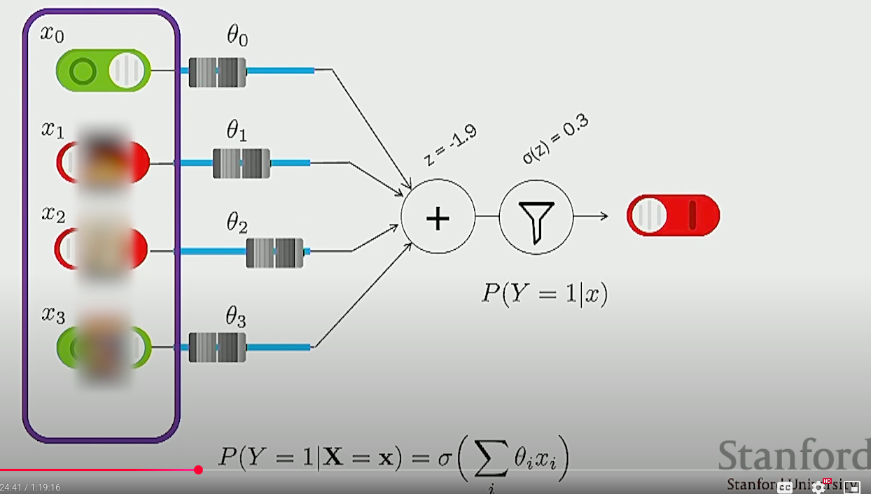
The logistic regression model is a discriminative $p (Y = y ∣ X = x; θ) \sim B er (p)$ with a decision boundary $k \in [0, 1]$ (in the case of $B er (p)$ , $k$ is usually set to $0.5$ so as to divide the mass by 2) that assumes that the parameter $p$ is affine with respect to $x$ . That is, $p (Y = 1 ∣ X = x) ⟹ p (Y = - 1 ∣ X = x) ⟹ p (Y = y ∣ X = x) = p := σ (w^{T} ϕ (x)) = 1 - p = 1 - σ (w^{T} ϕ (x)) = p^{y} (1 - p)^{1 - y} = σ (w^{T} ϕ (x))^{y} [1 - σ (w^{T} ϕ (x))]^{1 - y} [ϕ (x)_{0} = 1]$

where $σ : R \to [0, 1]$ is a non-linear function $σ := \frac{1}{1 + e x p ( - z )}$ , and where $w^{T} ϕ (x)$ is referred to as the logit since the inverse $σ^{- 1} := lo g \frac{p}{1 - p}$ is defined as the log odds ratio.

With the model now defined, the parameter $w$ needs to be estimated from the data $D = {(x^{(i)}, y^{(i)}) : (x^{(i)}, y^{(i)}) \sim iid X \times Y}_{i = 0}^{n}$ . This is done by using the negatve log likelihood as the loss function $L : R^{n} \to R$ to minimize so that $L (w) := - lo g \prod_{i = 1}^{n} p (y^{(i)} ∣ x^{(i)})$ is fixed with respect to the data $(x^{(i)}, y^{(i)})$

$\hat{w}_{M L E} \in argmin L (w) = argmin - i = 1 \sum n lo g σ (w^{T} ϕ (x^{(i)}))^{y^{(i)}} [1 - σ (w^{T} ϕ (x^{(i)}))]^{1 - y^{(i)}} = argmin - i = 1 \sum n y^{(i)} lo g σ (w^{T} ϕ (x^{(i)})) + (1 - y^{(i)}) lo g σ (w^{T} ϕ (x^{(i)}))$

where todo kl->ce.

where $argmin$ is implemented by first evaluating the gradient $\nabla L (w)$ and then iteratively applying gradient descent for each time step $t$ , $w^{(t + 1)} := w^{t} - α \nabla L (w)$ .

First, to evaluate the gradient, $\nabla L (w)$ , the negative log likelihood as loss function is simplified by defining $\overset{y}{^}^{(i)} := σ (w^{T} ϕ (x^{(i)}))$ so that $\nabla L (w) = - \sum_{i = 1}^{n} y^{(i)} lo g \overset{y}{^}^{(i)} + (1 - y^{(i)}) lo g \overset{y}{^}^{(i)}$ . Note that $\overset{y}{^}$ is not the target label but the probability of the target label. Then, since the derivative is linear with the derivative of the sum is the sum of the derivatives where $\frac{\partial}{\partial w} \sum_{i = 1}^{n} f (w) = \sum_{i = 1}^{n} \frac{\partial}{\partial w} f (w)$ , taking the derivative for a single example $i \in {1, \dots, n}$ for a single parameter $w_{j}$ where $L (w) = y lo g \overset{y}{^} + (1 - y) lo g \overset{y}{^}$ looks like

$\frac{\partial L ( w )}{\partial w _{j}} = \frac{\partial L ( w )}{\partial y ^} \frac{\partial y ^}{\partial w _{j}} = \frac{\partial L ( w )}{\partial y ^} \overset{y}{^} (1 - \overset{y}{^}) ϕ (x)_{j} = [\frac{y}{y ^} - \frac{1 - y}{1 - y ^}] \overset{y}{^} (1 - \overset{y}{^}) ϕ (x)_{j} = [\frac{y ( 1 - y ^ ) - y ^ ( 1 - y )}{y ^ ( 1 - y ^ )}] \overset{y}{^} (1 - \overset{y}{^}) ϕ (x)_{j} = [y (1 - \overset{y}{^}) - \overset{y}{^} (1 - y)] ϕ (x)_{j} = (y - \overset{y}{^}) ϕ (x)_{j} [by chain rule] [by \frac{d σ}{d z} = σ (1 - σ)] [by \frac{d l o g ( x )}{d x} = \frac{1}{x}]$

and so the evaluating the derivative of all examples $\nabla L (w) = - \sum_{i = 1}^{n} y^{(i)} lo g \overset{y}{^}^{(i)} + (1 - y^{(i)}) lo g \overset{y}{^}^{(i)}$ where $\overset{y}{^}^{(i)} := σ (w^{T} ϕ (x^{(i)}))$ looks like

$\frac{\partial L ( w )}{\partial w _{j}} = - i = 1 \sum n \frac{\partial}{\partial w _{j}} [y^{(i)} lo g \overset{y}{^}^{(i)} + (1 - y^{(i)}) lo g \overset{y}{^}^{(i)}] = - i = 1 \sum n (y^{(i)} - \overset{y}{^}^{(i)}) ϕ (x^{(i)})_{j} = - i = 1 \sum n (y^{(i)} - σ (w^{T} ϕ (x^{(i)}))] ϕ (x^{(i)})_{j}$

And so the swapping indices $j$ for the entire gradient gives $\nabla L (w) = - \sum_{i = 1}^{n} (y^{(i)} - σ (w^{T} ϕ (x^{(i)}))] ϕ (x^{(i)})$ . Recall now that the second step in implementing $argmin$ after taking $\nabla L (w)$ is to then iteratively apply gradient descent for each time step $t$ , $w^{(t + 1)} := w^{t} - α \nabla L (w)$ .

SITP